Differential graph computation
I recently received an email asking if differential dataflow might be a good fit for breadth-first search in evolving graphs. I think it is a great fit, and I pushed a breadth-first search example to the differential dataflow repository in my delight and satisfaction.
Around the same time I got a different email, asking if the recent CellIQ paper from NSDI, which does incremental connected components, is fundamentally new or might their “GStream” API be easily cast in something like timely dataflow or differential dataflow.
Now, I suspect this person was just a disgruntled trouble-maker. The GStream API (Listing 2) is clearly covered by differential dataflow, which allows arbitrary incremental updates to iterative computations containing operators like join and group_by, enough for many data-parallel graph computations. Whether it can be done is different from whether it can be done well, though.
The CellIQ paper is one step ahead of us, and observes that although graph computation can be expressed “using join and group_by, this can be very inefficient”, because “join operators are not optimized for graph processing and can be very expensive.” They then cite some papers which, perhaps coincidentally, try to sell you their special-purpose graph processors.
These authors are not wrong: it can be very inefficient and expensive, especially if you use a previous-generation platform not designed from the ground up to handle streaming iterative computation.
Let’s see what happens if you build on something better, using just join and group_by, of course.
Differential dataflow
Differential dataflow is a way of implementing data-parallel dataflow computations so that work is done only in response to changes in the data. If you change one input to your computation, you would prefer not to re-evaluate the entire computation. Rather, changes to the input produces some changes in the output of your first dataflow operator, which are then changes to the inputs of subsequent operators. Eventually these changes either evaporate or spill out the end of your dataflow as changed outputs.
Chasing these changes and doing only this work is what differential dataflow does well.
Importantly—and as far as we are aware, uniquely—differential dataflow also maintains this property in the context of iterative dataflow computations.
Going through the math for this usually results in long-lasting head-aches for the readers, so I’ll summarize instead. As changes flow around the dataflow, they “happen” at various logical times. These times reflect the epoch of streaming input data, and iteration counters for any loops they may be contained in. Rather than eagerly aggregate these changes, we leave them disaggregated, allowing future computation to use arbitrary subsets of the changes. Although we leave ourselves more work to do for each change, we end up with an orders-of-magnitude reduction in the numbers of changes.
We might be getting ahead of ourselves with detail. Let’s step back and set some context.
Data-parallel dataflow
The big-data-scenti have caught up with the idea that we should use high-level programming constructs to describe data-parallel computations. Two operators I’ll detail are group_by and join.
Warning : I’m going to over-simplify some of the operators in the coming sections. I recommend checking out the code for the real details, some of which are smart and some of which are gross.
Group By
The group_by operator acts on a collection of records. I’ll imagine a type Stream<D> to indicate a not-yet-fully-formed data collection of records of type D. In this setting, group_by has the following sort of signature:
fn group_by<K, V, F, R>(inp: Stream<(K,V)>, red: F) -> Stream<R>
    where F: Fn(&K, &[V], &mut Vec<R>);
For those of you familar with map and reduce, the group_by function is basically like reduce. The operator acts on a stream of key-value pairs, groups incoming pairs by their key value, and applies the reduction function red to each non-empty pair of key and matching records.
They way I’ve done this, it gets a mutable vector of elements R and it is supposed to write into them. I’m open to other suggestions. It turns out that writing tasteful interfaces to performant code is hard.
Join
The second important (for this post) data-parallel operator is join, a binary operator matching pairs of input records with the same key.
fn join<K, V1, V2>(in1: Stream<(K,V1)>, in2: Stream<(K,V2)>) -> Stream<(K,V1,V2)>;
The join operator is bi-linear, which means it has some nice mathematical properties (roughly: each input can be processed record-at-a-time, oblivious to other records from the same input).
Other operators
So I lied. We are going to add some more simple operators such as map, filter, and concat. These operators do not involve any data movement or grouping, and can always be performed in situ. They are also linear, and consequently do not need any special differential dataflow implementation.
Prelude: Bread-first search
Let’s use what we have so far start to build up an example of breadth-first search.
Our approach will be to maintain a stream dists of pairs (node, dist), indicating that node can be reached using dist edges. From a supplied set of edges edges, we want to expand this set by one hop: each node provides the distance in which it can be reached to each of its neighbors, who then retain the smallest distance they’ve seen. I’m going to use u32s for node identifiers. Sorry.
Our code follows this intuition, by using a join to provide the per-node information to neighbors. Under the covers, join maintains a list of key-value pairs as a trie: a flat list of keys, each with an offset into a flat list of values. Ignoring than the fact that these lists might change, this is the same as the adjacency list representation of a graph.
The output of join then needs to go through a map to increase the proposed distances by one.
To the proposals produced by join we concat the original distances. You might want one of those.
Finally, we use group_by to collect the distance proposals. Here I’m going to cheat and use the fact that my implementation of differential dataflow sorts records in each group (an important part of “consolidation”; details later). To find the least distance, we can just pop the first distance in the sorted order; we are guaranteed one exists, because we wouldn’t have been called if there was no data.
fn step(dists: &Stream<(u32, u32)>,
        edges: &Stream<(u32, u32)>) -> Stream<(u32, u32, u32)> {

    dists.join_u(&edges)
         .map(|(_, l, d)| (d, l+1))
         .concat(&dists)
         .group_by_u(|_, s, t| t.push(s[0]))
 }
You might have noticed that join_u and group_by_u each have a _u suffix. Rust doesn’t think highly of operator overloading, and so you need to have distinct method names if you would like to have distinct implementations. In this case, we are using an implementation that knows we have unsigned integer keys, and can use a more efficient index (a Vec rather than a HashMap).
Iterative data-parallel dataflow
We need one more operator. A different kind of operator. A higher-order operator: we need iterate.
The iterate operator has a simple signature (these higher-order things always do, don’t they?)
fn iterate<D, F: FnOnce(Stream<D>)->Stream<D>>(s: Stream<D>, f: F) -> Stream<D>;
The operator takes a stream, and a description of how to act on the stream. Its output is the result of acting on the input stream in the supplied manner a very large number of times.
Of course, since iterate just takes a description of what to do repeatedly, it doesn’t define any data movement or new computation itself. In actual fact, we will need a few helpers behind the scenes to tell just when we can stop computing, but we don’t need to detail them to understand what iterate is supposed to produce.
The iterate operator is incredibly important for efficient computation. It explains to your computer that you plan to do the same thing multiple times, and that it might be a good idea to spend a bit of effort to take advantage of that. Although you can do graph computation by repeatedly invoking join and group_by, you are doing your computer a disservice if you treat the invocations as unrelated.
Breadth first search
The combination of iterate with our step function produces a breadth-first search implementation.
The only non-obvious step is that the edges stream needs to be brought in to the body of iterate. This is not easy to do automatically (at least, not at the moment), and so we explicitly do this with the help of a stream that is inside the iterative context: dists.
// iteratively expand distances
roots.iterate(|dists| {
    step(&dists, &dists.context().enter(&edges))
}
In the fullness of time it may make sense for iterate to take a function of two parameters, a stream like dists and some sort of context object that does the things we had to ask dists to do for us.
That doesn’t really look all that complicated, does it? Now, we don’t yet know very much about what differential dataflow is doing under the covers, but that doesn’t have to stop us from grabbing the code and running it.
ALL SYSTEMS GO!!!
I turned this on with 500M edges and 100M nodes, using nodes 0, 1, and 2 as roots (so the distances are the distances from any of these three nodes). I then asked it to update (randomly re-wire) one edge per second, so that I could see how long updates take. If you do the same thing, you’ll see some output that looks like:
520.00s: observed at (Root, 520): 2 changes; elapsed: 0.004067797010065988s
522.00s: observed at (Root, 522): 2 changes; elapsed: 0.003325369005324319s
524.00s: observed at (Root, 524): 2 changes; elapsed: 0.002495013002771884s
526.00s: observed at (Root, 526): 2 changes; elapsed: 0.0021344090055208653s
527.00s: observed at (Root, 527): 2 changes; elapsed: 0.00011885000276379287s
532.00s: observed at (Root, 532): 2 changes; elapsed: 0.0019779420108534396s
541.00s: observed at (Root, 541): 2 changes; elapsed: 0.0032094839989440516s
545.00s: observed at (Root, 545): 3 changes; elapsed: 0.0020695959974545985s
548.00s: observed at (Root, 548): 2 changes; elapsed: 0.0017733170097926632s
553.00s: observed at (Root, 553): 2 changes; elapsed: 0.001985581999178976s
577.00s: observed at (Root, 577): 1 changes; elapsed: 0.0019018270104425028s
This tells us a few things: first, it takes about 500s to get the computation up and running. That is a lot of time to do BFS. We are spending time laying out the graph in a nice fashion, getting reading for incremental updates, all that stuff. I’m not going to try and defend this as good performance.
Did I mention this was single-threaded? It goes faster with more cores and computers. I’m pretty sure.
Once we start going we see that each incremental update (one random edge removal and addition) happens pretty quickly (the numbers over on the right). Most of these are single-digit milliseconds.
You might also notice that we miss some epochs; the node distances don’t always change, and in those cases we don’t print anything. They also go fast, but we don’t want to pat ourselves on the back just because the data didn’t change.
Graph connectivity
Way back when, someone said doing graph computation using join and group_by was inefficient.
Let’s return to that, shall we?
Graph connectivity is usually done with an algorithm very similar to BFS. Rather than propagate a distance that we increase by one, we propagate a set of labels (the same set as the node identifiers), and each node keeps the smallest label it sees. The only difference from BFS is that we start each node with its own label, rather than a few roots with distance zero (and we don’t add one to anything).
It turns out that this algorithm is horrible. We should all stop using it. Even graph-processing experts.
The algorithm is dumb because we start circulating all labels, even very large labels that will eventually get dominated by smaller labels. This is a waste of everyone’s time.
Improving with prioritization
A better algorithm, from at least as far back as the PrIter paper, is to start circulating small labels first, and move on to larger labels only once nodes have gotten a chance to see if they should bother proposing their name as a label. If they see a better label in the meantime, they don’t.
You can do this in differential dataflow with a fancier version of enter, that method that brought our set of edges in to the loop. We have an enter_at method that lets you specify a function from record to iteration number, and the record first gets added to resulting collection at that iteration number. This lets us write clever things like:
let nodes = inner.context().enter_at(&nodes,
    |r| 256 * (64 - r.as_usize().leading_zeros() as u32));
What a mess. What this is saying is that we should introduce a record (here a node identifier) at an iteration equal to 256 times its base 2 logarithm. Why that number? It turns out it is a (provably) good trade-off between giving labels enough time to propagate and not using too many distinct batches. Each batch gets a 256 iteration head-start on the next batch, which grow in size geometrically.
This approach is a bit different from PrIter’s approach, which just says “start running and always use the smaller labels”. This works great in PrIter’s more ad-hoc setting, but we really need to be clear about which iteration is which for differential dataflow to work its magic.
Running things
Since graph connectivity is a bit different from BFS, in particular we have to symmetrize the graph before doing the propagation, we are going to use a different number of nodes and edges than above. I chose 20M nodes and 400M edges, generated randomly, because those numbers are pretty similar (in magnitude) to taking half of the vertices in the twitter_rv dataset (about 42M nodes and 1.5B edges).
It takes about 800s to compute the connectivity information. This is slower than fancy graph processing systems on the twitter_rv dataset, and we are only processing one fourth the data. The slowness can be partially explained by the fact that we are generating a bunch of random data, ingesting and sorting it, paging because reasons, and then doing graph connectivity using differential dataflow, which does math and stuff. Also, I just wrote this stuff last week and haven’t found a good profiler yet.
It is also worth pointing out that the 800s time is one thread, and the computation is inherently parallel. If I had a cluster I could tell you how well it parallelizes. Given that I don’t have a cluster (or a profiler) it might take a bit of love before it does, but it has been done before.
Anyhow, it would be interesting to see if it has similar performance to the graph processing systems, because it can totally do some things they can’t even approach.
Tell us what can it do, Frank!
So we have our 400M edge graph, and we want to change it. Maybe someone tweetled an instachat.
We’ll do this two ways, to get a good latency measurement and then a good throughput measurement. Specifically, let’s try changing one edge at a time, and then let’s try changing 1,000 edges at a time.
We get the following cumulative density functions for the response time (from change introduced until confirmation that all output changes produced) for randomly tweaking one and one thousand edges, respectively:
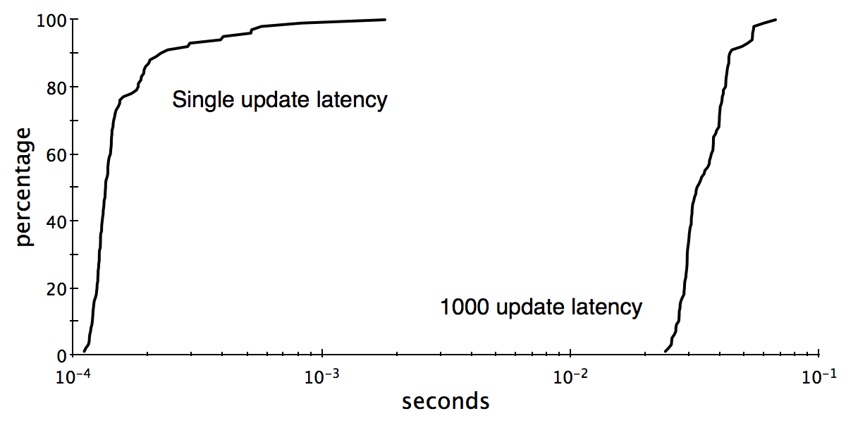
To explain, if we do one update at a time we get a median response time of 130 microseconds. If we do 1,000 updates at a time we get a median response time of 33 milliseconds. At this rate we should be able to do 30,000 edge updates per second, observing the correct graph connectivity output with a faster refresh rate than your favorite feature films.
The elapsed running times for graph connectivity are within striking distance of purpose-built graph processors running on clusters (stay tuned!), and we get near real-time interactive updates too boot.
Hey, and we did this all with just join and group_by (and iterate, to be fair). Who likes apples?
Up next: Under the covers
I’m going to try and explain differential dataflow again. It is pretty exhausting, but I think it is the sort of thing people need to understand if they want to work in the space of real-time graph analytics. I’ve got a bit of travel in the coming weeks, so in the meantime if you are keen you can totally check out the repo and lament the lack of intelligent comments and tests.
I’m hard at work tweaking the performance (mostly memory footprint) of differential dataflow. There are still a few cool things to do, and if you are interested in getting involved, let me know!