Worst-case optimal joins, in dataflow
I’ve gotten timely dataflow in Rust up and running exciting computations! I’m going to explain one that I think is especially cool, and that I’m going to try using for some performance analysis of the underlying system (the system has so far been subjected only to latency micro-benchmarks …).
The code for everything I’ll talk about is available online. It isn’t particularly pretty yet, but just you wait.
Seriously, you might actually want to wait. In the meantime, you can read this excellent post!
Relational Joins
A relational join is a pretty well studied thing, and I’m just going to lay some bare bones description here so that we have some common terminology. The problem starts with a collection of relations, think tables; we’ll call these relations . There are also several attributes, which we will refer to as . Each relation names some subset of these attributes, and each element in the relation has a value for each named attribute. Not all relations need to use the same set of attributes.
The relational join problem is, given several relations, determine the set of tuples over the full attribute space so that for each tuple, its projection onto the attributes of each relation exists in that relation.
An example
Consider the first records of the three relations , over the three attributes :
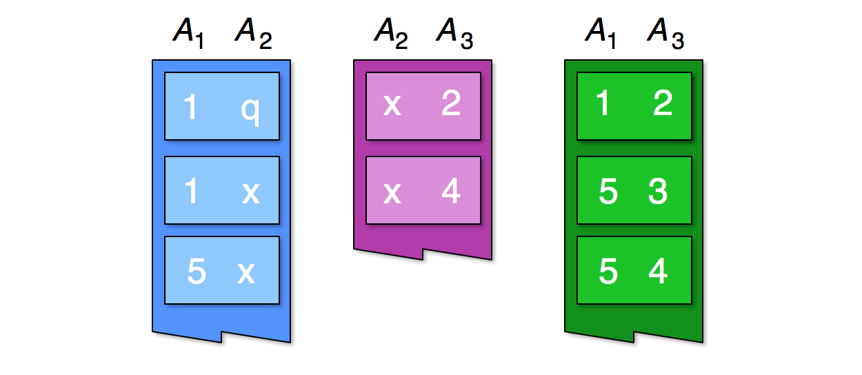
The relational join between the three relations must contains at least the triples and , because we can see in the first relation the pairs and , in the second relation the pairs and , and in the third relation the pairs and .
Of course, there may be more records in the full join as we see more of the records from each relation.
Ye Olde Methodologees
There are many ways to go about doing a binary join, between two relations, but the simplest is a hash-join, where you look at the attributes in common between the two relations and hash each tuple based on their restriction to those attributes. For each pair of matching tuples (one from each relation), you form the extended tuple that takes the union of the attributes of the relations.
In the example above, we might join the first two relations, by hashing records using the attribute . This matches and from the first relation with and from the second relation. The output data in this case are the four triples: , , , and . The record matches nothing in the second relation, and results in no output.
To do a multi-way join, one could just keep grabbing relations and joining them in, until all relations have been used. This gives the correct answer, but can be really slow. A smarter way is to form a “plan”, which is a binary tree in which the leaves are relations and the internal nodes correspond to joins of relations. The root of this tree is the join of all relations, but the tree structure suggests which relations are good to start joining together.
In the example above, we might prefer to join the three relations by first joining and , which would produce only two records before joining with . Building a smart join plan is something that database researchers like to talk about at their fancy meetings, and is a good way to strike up a conversation.
More recent work
Relational joins have been around for such a long while, you might be a bit surprised to learn that there is still new work going on here. You might be even more surprised to learn that, in some respects, folks have been doing it wrong for quite some time. This is exactly what Ngo et al observe, in awesome work:
-
The standard approach to computing relational joins, in which one repeatedly does binary joins, can do asymptotically more work than the join could ever possibly produce output tuples.
In the three-way join example, if each relation has size , there can be at most output tuples, because math. However, inputs exist so that any plan based on binary joins will do do work.
-
There exist algorithms that never do more work (asymptotically) than the join could, for some input of the same size, produce output tuples. For a three-way join, they will do computation.
This second point doesn’t mean that they will only do as much work as they will produce output tuples, only that when they do lots of work they at least have the excuse that they might have had to do it.
You know who doesn’t even have that excuse? The standard approaches to computing relational joins.
Generic Join
The algorithm that Ngo et al detail is really quite general. They even call the algorithm GenericJoin.
I’m going to focus on a specific realization of it. I should say at this point that the specific realization is due to other people, not me. I’m not really sure who gets credit, but Semih Salihoglu and Chris Ré are the ones that taught me about worst-case join processing, and it was with Semih, Chris, and Michael Isard that we banged out the first version of this in Naiad.
Specific Join
Rather than think of adding in relations one at a time, the way classical join processing might, we are going to think about adding in attributes one at a time.
Imagine we had the join on attributes , and want to output the join on attributes . For each we want to produce the set of supported by each relation .
The easiest way to do this is just to ask each : “what extensions do you support for ?” For each we intersect their results, and return for each in the intersection.
Of course, to ask the relations for the extensions and get the answer back quickly, each relation needs to be indexed by each prefix of attributes. This introduces redundancy, but we are going to work with it.
Smarter Join
Nothing about this algorithm is smart yet, but what Ngo et al observe is that if you do this intersection carefully, you get a worst-case optimal join algorithm. The specific care you have to take is, for each , only do work proportional to the smallest set of candidate extensions from any relation . Rather than just intersect everything willy-nilly, we have to start with the smallest and work our way up.
Fortunately, computing the intersection of a small set with a large set is something that can take time roughly linear in the size of the smaller set. You can either hash everything all over the place, or eat a logarithmic factor (they are ok with that) using various binary search techniques.
But, let’s look for a second and make sure we understand this. For each we have to ask a data-dependent relation to propose some extensions, and then ask the other relations to validate them. There isn’t a static plan saying “everyone first ask , then , then ..”; rather than pipeline records through relations, like a traditional join plan might, we are going to exchange them all over the place.
“Exchange”, you say? I hope you can see where this is going.
A Rust implementation
Obviously we were going to do this. Don’t act surprised.
Some abstractions
Do we really want relations and tuples all over the place in our code? No! Let’s do some abstraction.
From the discussion above we can see that we really only need a few things from a relation:
- It should be able to report how many extensions it would propose for .
- It should be able to propose specific extensions for .
- It should be able to intersect proposed extensions for with its extensions.
So let’s write a trait that does this. I’m going to call the tasks above “count”, “propose”, and “intersect”.
pub trait PrefixExtender<Prefix, Extension> {
    fn count(&self, &Prefix) -> u64;
    fn propose(&self, &Prefix) -> Vec<Extension>;
    fn intersect(&self, &Prefix, &mut Vec<Extension>);
}
I think this is as promised. This is what a relation needs to implement for us to be able to extend an element of type Prefix (think tuples ) with an element of type Extension (think ).
Distributed implementation
Of course, what we would really like is to extend each of the prefixes in parallel across many workers. At least, that is what I want. If you couldn’t care less, you should totally just skim this part.
To make this happen I’m going to use the timely dataflow libary, which uses a Stream<G, Prefix> type to represent a distributed stream of records of type Prefix. The G type parameter describes how the stream is distributed and how the computation will execute, and we’ll just ignore it for now.
We need to lift the implementation of a PrefixExtender<P, E> to work on streams Stream<G, P>.
Fortunately, I’m going to do this for us, by implementing the following trait for any type implementing PrefixExtender<P, E> (plus some information about how to distribute the prefixes among workers).
pub trait StreamPrefixExtender<G, P, E> {
    fn count(&self, &mut Stream<G, (P, u64, u64)>, u64) -> Stream<G, (P, u64, u64)>;
    fn propose(&self, &mut Stream<G, P>) -> Stream<G, (P, Vec<E>)>;
    fn intersect(&self, &mut Stream<G, (P, Vec<E>)>) -> Stream<G, (P, Vec<E>)>;
}
The records carry more information around with them; information that used to be on the stack now needs to be put in the records themselves. For example, we indicate the relation with the least count by a triple (prefix: P, count: u64, index: u64), data that would otherwise be in local variables. The signature of count is also changed to take and produces triples, like updating stack variables.
Although we are going to use this interface, you don’t need to know too much about about this. The main thing to know is that there are about fifty fairly predictable lines of code that go and implement a StreamPrefixExtender<G, P, E> for any type implementing PrefixExtender<P, E>.
impl<G, P, E, PE> StreamPrefixExtender<G, P, E> for Rc<RefCell<PE>>
where PE: PrefixExtender<P, E> {
    // the library does this for you, you just implement PrefixExtender.
}
Technically speaking, you will also need to tell timely dataflow how to distribute the prefixes. This will depend on how you distribute your relation, and is something I’ll say more about in an upcoming post.
Specific Join in Rust
With these abstractions, we are now ready to build a layer of the specific join algorithm. Before we do, let’s see what that would mean.
pub trait SpecificJoinExt<G, P, E> {
    fn extend(&mut self, extenders: Vec<Box<StreamPrefixExtender<G, P, E>>>)
        -> Stream<G, (P, Vec<E>)>;
}
We need to write a method for Stream<G, P> that, given a vector of arbitrary things implementing the StreamPrefixExtender<G, P, E> trait, produces a stream of pairs (P, Vec<E>). Also, we have to do it in the smart way described above, otherwise we’ll go slow like all the creaky database systems.
I’m just going to show you the code, but the comments should talk you through it. It’s just like we said.
impl<G, P, E> SpecificJoinExt<G, P, E> for Stream<G, P> {
    fn extend(&mut self, extenders: Vec<Box<StreamPrefixExtender<G, P, E>>>)
            -> Stream<G, (P, Vec<E>)> {

        // start with horrible proposals from a non-relation
        // ask each extender to try to improve each proposal
        let mut counts = self.select(|p| (p, 1 << 63, 1 << 63));
        for index in (0..extenders.len()) {
            counts = extenders[index].count(&mut counts, index as u64);
        }

        // for each of the extenders ...
        let mut results = Stream::empty();
        for index in (0..extenders.len()) {
            // find the prefixes the extender "won" the right to extend
            let mut nominations = counts.filter(move |p| p.2 == index as u64)
                                        .select(|(x, _, _)| x);

            // get the extensions and ask each other extender to validate
            let mut extensions = extenders[index].propose(&mut nominations);
            for other in (0..extenders.len()).filter(|&x| x != index) {
                extensions = extenders[other].intersect(&mut extensions);
            }

            // fold surviving extensions into the output
            results = results.concat(&mut extensions);
        }

        return results;
    }
}
This is the whole algorithm. It is really not super complicated. Rather, that is one layer of the algorithm.
To fill out a full relational join we need to call extend multiple times, with different PrefixExtender objects wrapping the same relations, just for different lengths of prefix. Let’s do an example.
A low-latency triangle enumerator
If we define a graph as a set of pairs (src, dst), a triangle is defined as a triple (a,b,c) where (a,b), (b,c), and (a,c) are each in the set of pairs. We can think of the triangles query as a relational join over three relations, which are the same data just bound to different pairs of attributes.
Defining a PrefixExtender
We will represent a fragment of graph by a list of destinations and offsets into this list for each vertex. For each interval, we will keep the destinations sorted to make the intersection tests easier.
pub struct GraphFragment<E: Ord> {
    nodes: Vec<usize>,
    edges: Vec<E>,
}
We’ll just write a quick helper function to let use get at the edges associated with a node:
impl<E: Ord> GraphFragment<E> {
    fn edges(&self, node: usize) -> &[E] {
        if node + 1 < self.nodes.len() {
            &self.edges[self.nodes[node]..self.nodes[node+1]]
        }
        else { &[] }
    }
}
It is worth pointing out that Rust is doing some very clever things under the hood here. It notices that we are returning a reference to some memory, the type &[E], and that the only thing this could refer to is &self. Rust then sets up the lifetime bound for the output to be that of &self and will ensure that when we use the result it is not allowed to out-live self itself.
I’m going to lie a little and present a simplified sketch of the PrefixExtender for GraphFragment. The simplified version uses a reference-counted GraphFragment, all that Rc<RefCell<...>> stuff. This allows us to have just one copy of the graph loaded and to share it out between folks who need it. We also need a helper function of type L: Fn(&P)->u64 to extract a node identifier from the type P.
impl<P, E, L> PrefixExtender<P, E> for (Rc<RefCell<GraphFragment<E>>>, L)
where E: Ord, L: Fn(&P)->u64 {
    // counting is just looking up the edges
    fn count(&self, prefix: &P) -> u64 {
        let &(ref graph, ref logic) = self;
        let node = logic(&prev.0) as usize;
        graph.borrow().edges(node).len() as u64
    }

    // proposing is just reporting the slice back
    fn propose(&self, prefix: &P) -> Vec<E> {
        let &(ref graph, ref logic) = self;
        let node = logic(prefix) as usize;
        graph.borrow().edges(node).to_vec()
    }

    // intersection 'gallops' through a sorted list to find matches
    // what is "galloping", you ask? details coming in just a moment
    fn intersect(&self, prefix: &P, list: &mut Vec<E>) {
        let &(ref graph, ref logic) = self;
        let node = logic(prefix) as usize;
        let mut slice = graph.borrow().edges(node);
        list.retain(move |value| {
            slice = gallop(slice, value); // skips past elements < value
            slice.len() > 0 && &slice[0] == value
        });
    }
}
That was pretty easy, huh? It sure was a lot messier before I wrote that edges(node) helper method. It is also a bit grottier when I’m not lying about how things work, but let’s not let that get between us.
In the interest of completeness (and eyeballs on my code) let’s look at the implementation of gallop. From an input slice and value, it skips forward in exponentially increasing steps, and then once it would overshoot the target value it moves forward in exponentially shrinking steps.
// advances slice to the first element not less than value.
pub fn gallop<'a, T: Ord>(mut slice: &'a [T], value: &T) -> &'a [T] {
    if slice.len() > 0 && &slice[0] < value {
        let mut step = 1;
        while step < slice.len() && &slice[step] < value {
            slice = &slice[step..];
            step = step << 1;
        }

        step = step >> 1;
        while step > 0 {
            if step < slice.len() && &slice[step] < value {
                slice = &slice[step..];
            }
            step = step >> 1;
        }

        &slice[1..]   // this shouldn't explode... right?
    }
    else { slice }
}
The gallop method can use any slice as input, and we give it a slice cut out of the graph’s edge list. If we mis-use the result slice there could be a horrible risk of aliasing, data races, de-, or re-allocation. Rust can confirm that none of this happens and just lets us use the same memory. It does this through retain’s closure, through a method I wrote (gallop), and through lots of weird logic. This is great!
Building the triangles query
So to recap, we have an implementation of PrefixExtender<P,E> whenever we have a combination of GraphFragment<E> and L: Fn(&P)->u64. This second part, the function, is what tells us how to turn a prefix P into an integer we can use to look up extensions in the graph. We use the same graph data everywhere, but fake out multiple relations by letting the function from prefix to attribute vary.
That being said, let’s count some triangles! We’ll do this in parts. I’m going to lie a bit again, and present some simplifications. Nothing horrible, just possibly mysterious things that would require a diversion to rationalize (and may just be bad design on my part).
First we just write some code that from a Communicator, which indicates a worker’s index and its number of peers, figures out what fragment of the graph this worker will load up and be responsible for. The code then prepares a dataflow computation and an input into which we will feed a: u32 values. This is all timely dataflow boiler-plate, and not super exciting from an algorithmic point of view.
fn triangles<C, F>(communicator: C, graph_source: F)
where C: Communicator,
      F: Fn(u64,u64)->GraphFragment<u32> {

    // load up the slice of graph corresponding to our index out of peers.
    let graph = graph_source(communicator.index(), communicator.peers());
    let graph = Rc::new(RefCell::new(graph));

    // prepare a new computation with one input.
    let mut computation = new_computation(communicator);
    let (mut input, mut stream) = computation.new_input();
The next step is to create the extender from a to (a,b). We just need to pair a copy of graph with a function that converts from a into a graph node identifier, and it will propose the adjacent b values.
//  // define an extender that uses 'a' to suggest x: '(a,x)' extensions
    let ext_b = vec![Box::new((graph.clone(), |&a| { a as u64 }))];
    let mut pairs = stream.extend(ext_b).flatten();
That flatten() method simply converts a Stream<G, (P, Vec<E>)> to a Stream<G, (P, E)>. It is just 17 lines of code somewhere, so hooray for timely dataflow being easy to use (succint, at least).
The next step is to create the extenders from pairs (a,b) to triples ((a,b),c). There are going to be two extenders, as we want values c such that both (a,c) and (b,c) are present in the graph. Each extender needs to take an (a,b) and identify an edge source, and there only two choices.
//  // define extenders using 'a' and 'b' to suggest x: (a,x) and x:(b,x)
    let ext_c = vec![Box::new((graph.clone(), |&(a,_)| { a as u64 })),
                     Box::new((graph.clone(), |&(_,b)| { b as u64 }))]

    let mut triangles = pairs.extend(ext_c).flatten();
Let’s also take a peek at what we see, printing out the triangles (observe is another 16 lines of code).
//  // take a peek at what gets produced.
    triangles.observe(|&tri| println!("triangle: {:?}", tri));
Ok, we’ve got the data loaded up, the computation defined, and are ready to go. Let’s triangularate!
//  // finalize dataflow structure
    computation.0.borrow_mut().get_internal_summary();
    computation.0.borrow_mut().set_external_summary(Vec::new(), &mut Vec::new());

    // introduce u32s to find triangles rooted from them
    for node in (0..graph.borrow().nodes.len()) {
        input.send_messages(&((), node as u64), vec![node as u32]);
        input.advance(&((), node as u64), &((), node as u64 + 1));
        computation.0.borrow_mut().step();
    }

    // close input and finish any computation
    input.close_at(&((), graph.borrow().nodes.len() as u64));
    while computation.0.borrow_mut().step() { }
}
This runs through each possible source node and produces all triangles starting from that vertex.
Didn’t you say “low-latency”?
Good point. Although we went through all nodes in order, to enumerate all triangles, we didn’t have to. We could just as easily have written the main loop as:
for epoch in (0..) {
    let node = read_u32_from_console(); // not a real function!
    input.send_messages(&((), epoch), vec![node]);
    input.advance(&((), epoch), &((), epoch + 1));
    computation.0.borrow_mut().step();
}
This reads input in from the user, fires that off to the dataflow, which prints out observed triangles asap. To give a sense for how promptly, let’s throw a timer in the standard loop up above, and start things up single-threaded on a fairly standard LiveJournal dataset:
Caveat: the code is barely tested and may be wrong; do not buy/sell anything based on these data.
enumerated triangles from (0..1) in 67947ns
enumerated triangles from (1..2) in 42738ns
enumerated triangles from (2..3) in 26064ns
enumerated triangles from (3..4) in 48006ns
enumerated triangles from (4..5) in 19921ns
...
So the time between injecting a node identifier and getting all the triangles back out is some tens of microseconds. These numbers get a little better with batching, cutting out some of the overhead:
enumerated triangles from (0..10) in 231301ns
enumerated triangles from (10..20) in 276721ns
enumerated triangles from (20..30) in 149940ns
enumerated triangles from (30..40) in 137285ns
enumerated triangles from (40..50) in 155781ns
...
And even better with even more batching, as it starts to look more like 10-15us amortized per vertex.
enumerated triangles from (0..1000) in 10129064ns
enumerated triangles from (1000..2000) in 12018695ns
enumerated triangles from (2000..3000) in 11323832ns
enumerated triangles from (3000..4000) in 11224684ns
enumerated triangles from (4000..5000) in 14810182ns
...
This program is meant to stress several components and reveal what is slow and needs some work. The underlying system still has lots of room to improve (I think).The numbers should only get better.
Triangles are soooo lame.
Triangles are so 2014! Everyone does triangles! Do something cooler!
// define extenders to add a 'd' coordinate connected to each of a, b, c.
let ext_d = vec![Box::new((graph.clone(), |&((a,_),_)| { a as u64 })),
                 Box::new((graph.clone(), |&((_,b),_)| { b as u64 })),
                 Box::new((graph.clone(), |&((_,_),c)| { c as u64 }))];

let mut quads = triangles.extend(ext_d).flatten();
In case you missed it, that was us defining a dataflow computation to enumerate 4-cliques.
enumerated 4-cliques from (0..1) in 164474ns
enumerated 4-cliques from (1..2) in 230093ns
enumerated 4-cliques from (2..3) in 40667ns
enumerated 4-cliques from (3..4) in 154921ns
enumerated 4-cliques from (4..5) in 67344ns
...
Not impressed? How about:
enumerated 5-cliques from (0..1) in 115570ns
enumerated 5-cliques from (1..2) in 311967ns
enumerated 5-cliques from (2..3) in 110915ns
enumerated 5-cliques from (3..4) in 126838ns
enumerated 5-cliques from (4..5) in 104806ns
...
What about:
enumerated 6-cliques from (0..1) in 107292ns
enumerated 6-cliques from (1..2) in 342537ns
enumerated 6-cliques from (2..3) in 93778ns
enumerated 6-cliques from (3..4) in 134948ns
enumerated 6-cliques from (4..5) in 87148ns
...
I can keep going (seriously, I wrote a program to do it).
Arbitrary graph motif finding (small subgraphs you want to find in a large graph) is really easy to write. I’m sure there is lots of smarter research on how to do it will, but this is worst-case optimal, at least.
Wrap-up
There is some seriously cool work going on in join research. It isn’t nearly as stale as I thought it was. But, importantly, these new algorithms need better systems than your bog-standard batch processors.
How many of your favorite graph processors are able to start handing back 6-cliques in less than a millisecond, with a memory footprint that is roughly just the graph itself? Not the one you use? Why not? Being bad at things stopped being cool in high school…
On the positive side, in addition to this code, Naiad can do all this, and Flink should be able to as well.
From my point of view, I now have a cool problem I can use to tune timely dataflow. I would expect it to start getting better and more usable (and I’ll probably actually try it in more configurations now too).
Footnote: Skew
One of the theoretical concerns about this sort of approach is how well it distributes in the presence of skew. Each of our count, propose, and intersect operators is “data-parallel”, but is this actually helpful when the data are themselves not uniformly distributed among workers.
The implementation I’ve talked about is not skew-resilient. If a vertex has a really high degree, all the edges may be placed on one machine. Adding more machines will not make propose go any faster, and will not prevent all proposals from being sent to this one machine for intersection.
However, you can whip together a skew-resilient version of each of these operations.
countis naturally skew resilient because we just need a number for each prefix. They can be distributed (uniformly) by a hash on the prefix.proposecan be made skew resilient by distributing the extensions for each prefix to machines sequentially from a machine identified by a hash of the prefix. We need to know how many machines to ask for extensions, but each proposal should come with a count (I dropped it; oops).intersectcan be made skew resilient by distributing the(P, E)records by hash, and shipping proposals to the known location for each relation.
I’m not intimate enough with the work in the area to know for sure that this ticks all of the desired boxes. For example, one desideratum is that the computation take few “rounds”, in the MapReduce sense. Given that I don’t use MapReduce and still get computation done, this doesn’t really bother me.
Flip comments aside, it would be good to understand if this approach does represent a scalable, skew-resilient worst-case optimal join algorithm. I’ve been told that this would be pretty cool.
Credits and on-going work
This area (worst-case optimal join processing) is super cool, and I owe a debt to Semih Salihoglu and Chris Ré for introducing the two of us. These folks and their colleagues are still very active, pushing the boundaries of what can be done to make join processing faster and faster.
Semih, Chris and others have an approach to make even more complex joins efficient by using hypertree decompositions of queries. “Tree-like” acyclic queries have knowns ways to process them optimally (Viterbi-style). Once you get cycles they break, but if you can decompose the query into a tree of small cyclic queries and use the worst-case optimal techniques on the cyclic queries you get some nice results.
Chris Aberger, Chris and others have a neat way to make the intersection testing much more efficient using SIMD instructions, and show that they can get orders-of-magnitude speed-ups by using these techniques. Various “unnamed” proprietary vendors seem to get well and thoroughly trounced.
There is plenty of other work I’m not as familiar with (yet), but it seems to just keep coming. Be excited!